Analyze RAP data in GEE

Purpose

This script identifies and summarizes trends in selected bands of RAP fractional cover products using the Mann-Kendall test to determine significance, and both Sen's slope and a simple linear regression to ascertain the annual rate of change and the estimated cumulative change over the entire time period of the analysis.

Step-by-step Instructions

1

Define or upload your shapefile with multiple regions of interest

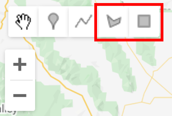
You can draw your region of interest using the GEE interactive map. You can do so by zooming to your general region of interest and then either drawing a free-hand polygon or a rectangle.

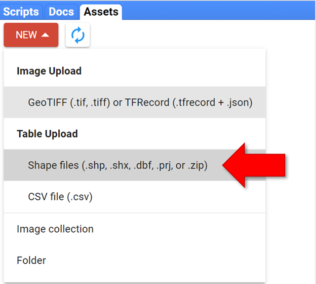
To upload, click on the Assets tab in the left-side window and then click the New button and select Shape files.

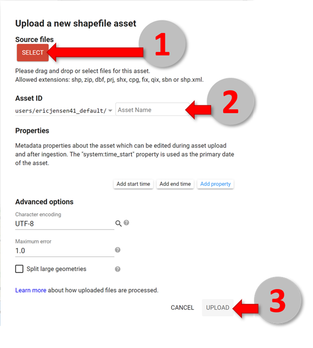
A pop-up window will open. Follow these steps: 1) Click the SELECT button and upload either a zipped shapefile or each of the file extensions separately (a zipped shapefile is usually easiest), 2) name your new Earth Engine Asset, and 3) leave the remaining items as default, and click UPLOAD.

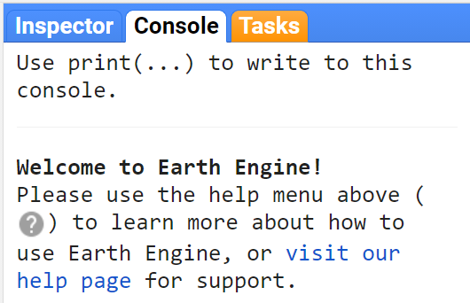
Upon initiating the upload, the Tasks tab in the right-side window will light up yellow, indicating that the upload has started.

Depending on the complexity of the shapefile geometry and the number of features, it may take several minutes or longer to complete.

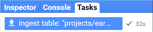
You can refresh the web page to see if it has finished. Once it lights up blue, the upload has completed.

Click on the Assets tab in the left-side window again. This time, find your new asset and click the arrow to import it.

You will now see a new import table at the top of your script.

Note: If your region is too large, you will receive an error!

Once you have created or uploaded and added your region, you will see a new import called “table” that you should rename to "geometry" at the top of the script by clicking its name.

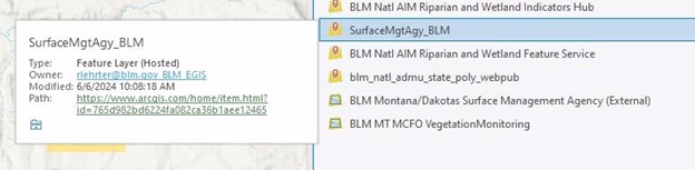
Optionally, you can draw or upload an additional shapefile to filter the rasters within your geometry. In this example, we will use a shapefile of BLM land ownership so our output only retains information for the BLM land within the geometry polygon. Specifically, we imported these BLM admin polygons: https://www.arcgis.com/home/item.html?id=765d982bd6224fa082ca36b1aee12465

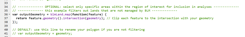
In order to run the script with the additional filter geometry, you will need to rename the polygons imported for filtering “blmLand”, uncomment lines 36-38, and comment out line 41 to resemble the screenshot below.

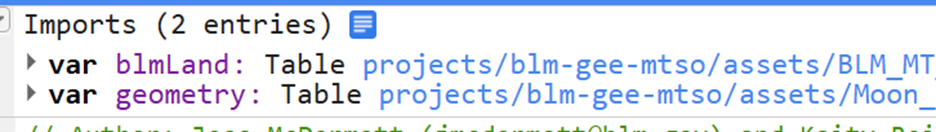
The imported assets at the top of your script should look like the screenshot below with the omission of blmLand if you are not using that step.

2

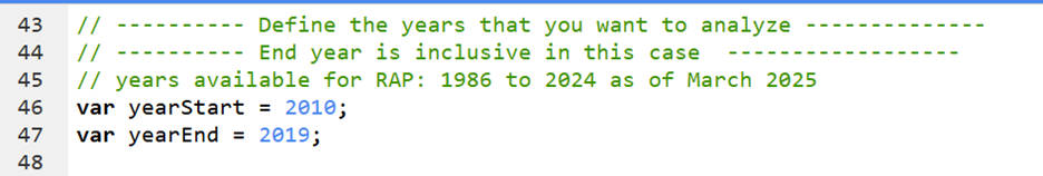
Define the years that you want to export

The yearStart and yearEnd variables on  lines 46 and 47 of the script define the first and last years of data that will be exported. The example below exports data for every year between 2010 and 2019.

To export multiple non-sequential years, simply run the script multiple times.

3

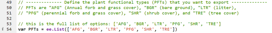
Define the plant functional types you want to export

The PFTs variable on line 54 of the script is a list of the plant functional types (PFTs) that you want to export. You can either keep the entire list if you want to export all of them or remove any PFTs that you are not interested in. 

'AFG' is annual forb and grass cover, 'BG' is bare ground cover, 'LTR' is litter cover, 'PFG' is perennial forb and grass cover, ' SHR' is shrub cover, and 'TRE' is tree cover.

4

Select confidence interval

Change the critical z value based on the desired confidence interval for masking out insignificant pixels. For example, the current default of 1.28 corresponds to a confidence interval of 80%, meaning we can be 80% confident that the true trend differs from zero when a pixel is considered significant (i.e., not masked in the output). Another common, more stringent critical z value is 1.96, which corresponds to a 95% confidence interval.

5

Choose your variables and output names

This script offers several different output rasters that represent trends of fractional cover over time. Sen's slope is a nonparametric analysis that is robust to outliers and non-normal data commonly found in ecological studies. It calculates the annual trend between each pair of subsequent years and selects the median of these slopes. Linear regression is a statistical method that fits a straight trend line to the data by minimizing the differences between observed and predicted values, assuming normality and being sensitive to outliers. The outputs from both analyses can be interpreted as follows: A positive value indicates an annual or cumulative increase in the % fractional cover of the selected vegetation bands, while a negative value signifies an annual or cumulative % decline. For example, an AFG_Annual_Sens_Slope or AFG_Annual_Trend of -2 would indicate that pixel is experiencing a decline of 2% fractional cover of annual vegetation per year on average over the selected years of analysis. In contrast, an AFG_Overall_Sens_Slope or AFG_Overall_Trend of -2 would indicate that pixel is estimated to have experienced a total decline of 2% fractional cover of annual vegetation over the entire period of analysis. Keep in mind there is nothing constraining the average and overall trend in this analysis, so you might get a trend estimate that is unrealistic (e.g., an increase of over 100% even though RAP cover cannot exceed 100%).

Comment lines on or off using a double forward slash “//” to select which variables you want to receive as output. By default, the sens slope per year and overall masked and unmasked are the only output.

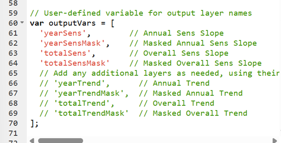
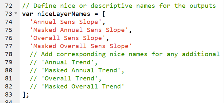
Be sure to comment the corresponding names on or off if you change the default layers output. You can also change the name of the layer here if you desire.

For example, if I wanted to include the annual trend as an output, I would add a comma after line 64 (‘totalSensMask’,), remove the // and comma from line 66 (‘yearTrend’). I would also perform a similar action to the niceLayerNames variable by adding a comma to line 77, then removing the // and comma from the corresponding name from that layer (line 79).

6

Run the script

Simply click "Run" at the top of the script to export your data, which will initiate the export process for each year of data.

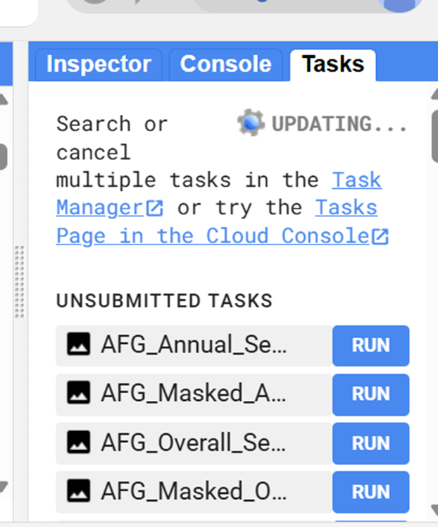
Almost immediately, the "Tasks" tab in the right-side panel will turn yellow indicating that you are ready to export. When you click "Tasks" you will see a list with items for each layer that you exported. Click "Run" on each of them to begin processing. You can click Run on the export popup to keep the default settings, which will export the raster as a geotiff to the Google Drive linked to your Google Earth Engine account.

7

Retrieve your output

The export process may take several minutes to complete. However, once you have started the export you can close the Earth Engine tab and it will continue to run. You can always return to the Tasks tab at code.earthengine.google.com to check on the progress of your export. Once your table has finished exporting you will find them in your Google Drive. It is now available for you to download to your local computer.

8

OPTIONAL: Retrieve summary statistics about your geometry of interest

The end of this script offers summary statistics about RAP over the time period of interest for your masked geometry (i.e., quartiles, mean, median). To run this portion of the code, you need to uncomment lines 262-376. Highlight those lines and use a keyboard shortcut (ctrl + /) to easily uncomment that section of code. Then you can run the code as usual and there will be a new output available for export- Chart_Data_Export.csv. That export contains annual summary statistics for your geometry over the years of interest. Scroll down in the console to see graphs made from those data. You may take a screenshot of that graph, but it cannot be exported directly at this time.

Note: This portion will not run if your area of interest is too large- it runs into memory issues!

9

OPTIONAL: Visualize your output raster(s) in ArcGIS Pro

Download your output raster(s) from Google Drive. Add the raster(s) to your ArcGIS Pro project by dragging and dropping into the Contents window or Add Data -> navigate to file(s) location. Allow it to calculate statistics if that pop-up window appears. You might notice your raster no longer appears to be clipped to your geometry of interest or masked by significance. For example:

Right click the newly added raster layer -> Symbology -> Mask -> Check Display background value -> add -9999 to the box below that check.

This step is necessary because GEE and ArcGIS Pro do not currently correctly communicate which values of the raster do not contain any data. Without completing this step, the clipped or masked areas of your raster will erroneously appear to be data in ArcGIS Pro. Your raster(s) output should appear as expected now: